Photos

Week 12: Arc Pad Data Collection

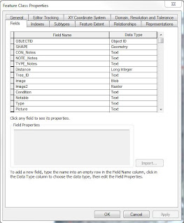Figure 12-1. Table showing all the attributes that we would collect in the field.

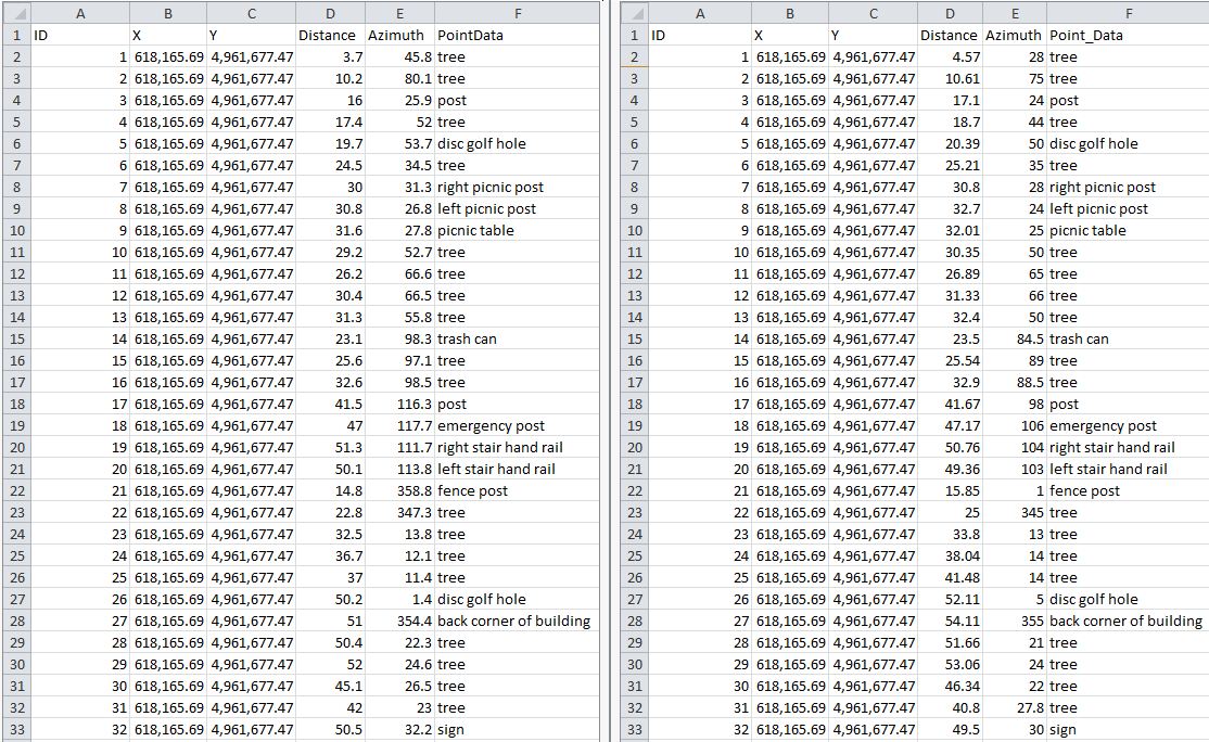
Figure 12-2. Table showing all the data we collected in the field.

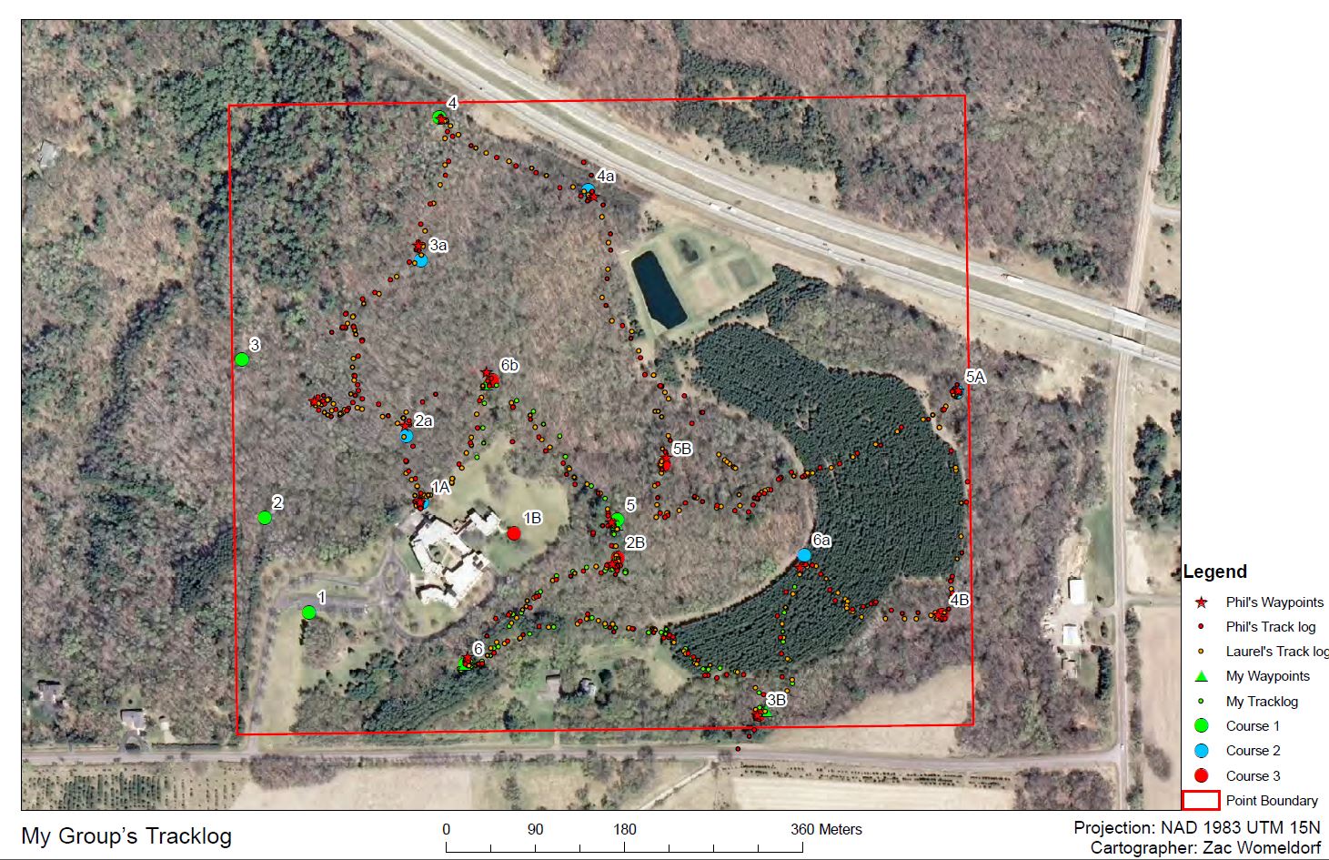
Figure 12-3. Map of all the Tree Types along the paths.

Figure 12-4. Map of notable trees along the Priory path.

Figure 12-5. Map of notable tree conditions along the Priory path.

Week 11: HABL Balloon Launch 

11-1. Us walking the balloon out to the launch point.

Figure 11-2. The balloons flight path for the first few minutes of the flight.

Figure 11-3. The general path of the balloon for the first about half hour of flight.

Figure 11-4. The complete path of the balloon for the entire flight. Origin is the green dot, red is the landing spot.

Figure 11-5. Good image of the Chippewa River bending around campus. Haas Arts Center is the building on the right.

Figure 11-6. Great image of the Eau Claire River.

Figure 11-7. An image of some nice cumulus clouds. Can see the condensation on the lens at this height

Figure 11-8. Image of the curvature of the earth, starting to see the blackness of 'outer space'.

Figure 11-9. Image showing the blackness of space at the top.

Figure 11-10. Image of our professor retrieving the rig and balloon remnants from the tree.

 Week 9: Balloon Mapping Part I

Figure 9-1. Initial Camera rig design.

Figure 9-2. A 50ft mark in the string.

Figure 9-3. Us filling up the balloon with helium. The tube runs from the tank to the balloon.

Figure 9-4. The balloon with all attachments. The white container houses the camera, the blue unit is a Garmin eTrex GPS, and that's me in the hat and black jacket holding the string reel.

Figure 9-5. The path us and our balloon took around campus. Note: There have been major changes to campus and the building we seemingly walk through is no longer there. I was unable to find a recently updated aerial image of UWEC.

Figure 9-6. Us launching the video camera rig.

Figure 9-7. Us avoiding tangling up with a lamp post.

Figure 9-8. Map of our route on campus for the video mapping.

Figure 9-9. A screenshot from my Map Knitter session.

Figure 9-10. My georeferencing session on ArcMap. You can see the georeference nodes in the corner of the overlaying image.

Figure 9-11. Image showing the balloon being at an angle to the ground instead of perpendicular.

Figure 9-12. Image captured from balloon of our new Student Union Building.

Figure 9-13. The balloon being reeled in and the rig being completely upside down.

Figure 9-14. The black tape signifying that 400ft of string had been released.

Figure 9-15. The balloon flying away after detaching from the string.

Figure 9-16. Mosaicked images in ArcMap. One can see the distortion at the edges of the images fairly easily, especially the buildings.

Week 8: Final GPS Navigation

Figure 8-1. Priory Locator. South of the City of Eau Claire

Figure 8-2. The paintball guns we were equipped with, along with Mask, Hopper and CO2 tank.

Figure 8-3. Map of my group member's track logs

Figure 8-4. Map of my track log, it ran out of battery.

Figure 8-5. Map of every group member's track log.

Figure 8-6. A basic description of a flank, I moved around the target and was able to subdue him.

Week 7: GPS Navigation

Figure 7-1. The table containing the points for each navigation course.

Figure 7-2. Image of Garmin eTrex unit.

Figure 7-3. Map of my group's navigation points.

Figure 7-4. Map of each group's navigation points.

Week 6: Navigation with Map and Compass

Figure 6-1. Chart of navigational points. We had Course #2.

Figure 6-2. Final navigation path with all points plotted. 1A is the starting point.

Figure 6-3. Point 4A is on the slope of the hill but hard to tell exactly where. The waste water area is the cluster polygons to the right of point 4A.

Figure 6-4. Me finding the azimuth of a path.

Week 5: Navigation and Map Construction

Figure 5-1. 2 ft. contour map of UWEC Priory.

Figure 5-2. 5 ft. contour map with aerial image of UWEC Priory.

Week 4: Distance Azimuth Survey

Figure 4-1. Campus the day we measured.

Figure 4-2. Example of measurement view for TruPulse 360.

Figure 4-3. Declination example. The declination is positive.

Figure 4-4. Table showing TruPulse measurements on left, Compass on right.

Figure 4-5. Final Result of Distance Azimuth Survey

Figure 4-6. First error in the Bearing Distance to Line tool.

Figure 4-7. Errors in the Nodes. Blue is the true locations.

Week 3: Balloon Project Beginning

Figure 3-1. Camera stabilized by string with rubber band holding down the capture photo button.

Figure 3-2. Weight Chart for Payload Materials

Figure 3-3. Parachute Test (For HABL) with Payload of 2 lbs.

Figure 3-4. Camera in Rig for Balloon Mapping.

Figure 3-5. Video of Parachute Test with Test Payload of 2 lbs.

Week 2: New and Improved Sandbox Exercise

Figure 2-1. Kriging interpolation

Figure 2-2. Spline Interpolation. The best representation of the first survey.

Figure 2-3. Natural Neighbor interpolation.

Figure 2-4. IDW interpolation.

Figure 2-5. Strings drawn across the length of the sandbox in 5 cm intervals.

Figure 2-6. Redone Point Feature Class with Spline interpolation underneath.

Figure 2-7. Spline interpolation. The best representation of the second survey.

Figure 2-8. Final image of terrain.

Week 1: Sandbox Exercise

Figure 1-1. Drew forming a depression in the realm

Figure 1-2. Me perfecting the river

Figure 1-3. Hannah documenting the x,y,z values

Figure 1-4. Me enjoying the -7 temperature

Figure 1-5.

Figure 1-6. Final Image of our terrain

Figure 1-7.A warm up break

Figure 1-8. Points plotted in ArcMap 10.